EigenFace

PCA

SVD

This notebook will dive into eigenvalues and eigenvectors with covariance matrix. We also compare this method with SVD to understand what happens under the hood.

Published

May 26, 2022

Import packages

%matplotlib inline
import matplotlib.pyplot as plt
import seaborn as sns
import numpy as np
import pandas as pd
from PIL import Image

Load data

X_train = np.loadtxt('../../../data/faces_train.txt')
y_train = np.loadtxt('../../../data/faces_train_labels.txt')
X_train.shape, y_train.shape

((280, 1024), (280,))

X_test = np.loadtxt('../../../data/faces_test.txt')
y_test= np.loadtxt('../../../data/faces_test_labels.txt')
X_test.shape, y_test.shape

((120, 1024), (120,))

Understand the data

sample = X_train[0]
sample.shape

(1024,)

X_train.shape[0] / 40

7.0

X_test.shape[0] / 40

3.0

Define a function to convert the data to image array and display the face images.

def show_images(arr, num_person, num_faces):
    data = arr[:num_person*10]
    fig, axs = plt.subplots(num_person, num_faces, figsize=(num_faces, num_person))
    flat_axs = axs.flatten()
    for i in range(num_person):
        for j in range(num_faces):
            flat_axs[i*num_faces+j].imshow(arr[i * int(arr.shape[0] / 40) + j].reshape(32, 32).T)
            flat_axs[i*num_faces+j].axis('off')
    plt.set_cmap('gray')
    plt.tight_layout()
    plt.show()

show_images(X_train, 3, 5)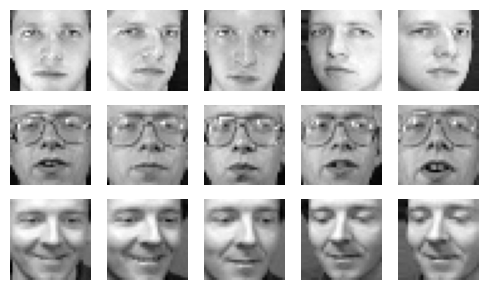

Show mean face

def show_image(data):
    fig, ax = plt.subplots(figsize=(1,1))
    ax.imshow(data.reshape(32, 32).T)
    ax.axis('off')
    plt.set_cmap('gray')
    plt.tight_layout()
    plt.show()

mean = X_train.mean(0) # shape (1024,)
show_image(mean)

Perform PCA from covariance matrix

Compute eigenvalues and eigenvectors of covariance matrix

def pca(data):
    mean = data.mean(0) # shape (1024,)
    Z = data - mean
    S = Z.T @ Z
    eigenvals, eigenvecs = np.linalg.eigh(S) # the eigen values are sorted from smallest to largest
    reversed_idx = np.argsort(-eigenvals) # get the reversed indices from the largest to smallest
    eigenvals = eigenvals[reversed_idx]
    eigenvecs = eigenvecs[:, reversed_idx]
    return eigenvals, eigenvecs

%%time
eigen_vals, eigen_vecs = pca(X_train)

CPU times: user 1.15 s, sys: 63.9 ms, total: 1.21 s
Wall time: 174 ms

eigen_vals.shape, eigen_vecs.shape

((1024,), (1024, 1024))

eigen_vals

array([ 7.59100215e+07,  4.19397005e+07,  2.54955933e+07, ...,
       -5.02190332e-09, -7.09703055e-09, -7.63365465e-09])

eigen_vecs[:5]

array([[-0.01287756, -0.05501646,  0.0041873 , ...,  0.        ,
         0.        ,  0.        ],
       [-0.01462181, -0.06097046, -0.00761386, ...,  0.04503731,
         0.06237077,  0.21112058],
       [-0.01704114, -0.06917858, -0.01997429, ...,  0.08273158,
         0.36417853,  0.14920292],
       [-0.02048617, -0.07692255, -0.02277752, ..., -0.04538269,
        -0.0119913 , -0.37879662],
       [-0.02213695, -0.07991882, -0.02080318, ...,  0.02432163,
         0.13519464,  0.02273907]])

Show top 5 eigenfaces

def show_pc_images(data):
    nrows, ncols = data.shape
    fig, axs = plt.subplots(1, ncols, figsize=(ncols, 1.5))
    flat_axs = axs.flatten()
    for i in range(ncols):
        flat_axs[i].imshow(data[:, i].reshape(32, 32).T)
        flat_axs[i].axis('off')
        flat_axs[i].set_title(f'pc{i}')
    plt.set_cmap('gray')
    plt.tight_layout()
    plt.show()

show_pc_images(eigen_vecs[:, :5])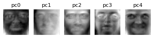

Perform PCA with SVD

def svd(data):
    data_centered = data - data.mean(0)
    U, s, Vt = np.linalg.svd(data_centered)
    return U, s, Vt.T

%%time
U, s, V = svd(X_train)

CPU times: user 837 ms, sys: 26.8 ms, total: 864 ms
Wall time: 124 ms

U.shape, s.shape, V.shape

((280, 280), (280,), (1024, 1024))

Note

V is the same as the eigen vector matrix, and \(s^2\) is equal to the corresponding eigen values.

Check if the top 5 eigenvalues are equal

np.square(s[:5]), eigen_vals[:5]

(array([75910021.54729882, 41939700.47489863, 25495593.34635307,
        17539063.72985784, 12170662.99105223]),
 array([75910021.54729888, 41939700.47489879, 25495593.34635304,
        17539063.72985789, 12170662.99105226]))

np.allclose(np.square(s[:5]), eigen_vals[:5])

True

Check if the top 5 eigenvectors are equal

V[:, :5], eigen_vecs[:, :5]

(array([[-0.01287756,  0.05501646,  0.0041873 ,  0.00651911,  0.0704008 ],
        [-0.01462181,  0.06097046, -0.00761386,  0.00091407,  0.07140231],
        [-0.01704114,  0.06917858, -0.01997429, -0.00113944,  0.0715405 ],
        ...,
        [ 0.00308199, -0.04617929, -0.03671734,  0.03130467,  0.07777847],
        [ 0.00747202, -0.0494147 , -0.04110058,  0.03836678,  0.07902728],
        [ 0.0109414 , -0.05125083, -0.03781413,  0.04223883,  0.07396954]]),
 array([[-0.01287756, -0.05501646,  0.0041873 , -0.00651911,  0.0704008 ],
        [-0.01462181, -0.06097046, -0.00761386, -0.00091407,  0.07140231],
        [-0.01704114, -0.06917858, -0.01997429,  0.00113944,  0.0715405 ],
        ...,
        [ 0.00308199,  0.04617929, -0.03671734, -0.03130467,  0.07777847],
        [ 0.00747202,  0.0494147 , -0.04110058, -0.03836678,  0.07902728],
        [ 0.0109414 ,  0.05125083, -0.03781413, -0.04223883,  0.07396954]]))

Tip

Since eigenvectors can be same values, but with opposite signs, we compare the absolute values.

np.allclose(np.abs(V[:, :5]), np.abs(eigen_vecs[:, :5]))

True

Show top 5 eigenfaces

show_pc_images(V[:, :5])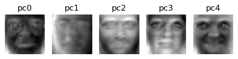

Projecting 3 persons’ faces data down to 2 dimensions and plot them.

T = X_train[:7*3, :] @ V[:, :2]
T.shape

(21, 2)

y = y_train[:7*3].reshape(-1, 1)
y.shape

(21, 1)

data_2d = pd.DataFrame(data=np.concatenate((T, y), axis=1), columns=['pc1', 'pc2', 'person'])
data_2d.head()

	pc1	pc2	person
0	-4907.496730	458.054067	1.0
1	-4344.197376	1289.734627	1.0
2	-4775.345055	577.090674	1.0
3	-4492.115417	-930.775823	1.0
4	-4639.398032	840.018975	1.0

fig, ax = plt.subplots(figsize=(8, 5))
sns.scatterplot(data=data_2d, x='pc1', y='pc2', hue='person', palette=['blue', 'red', 'green'], ax=ax)
plt.show()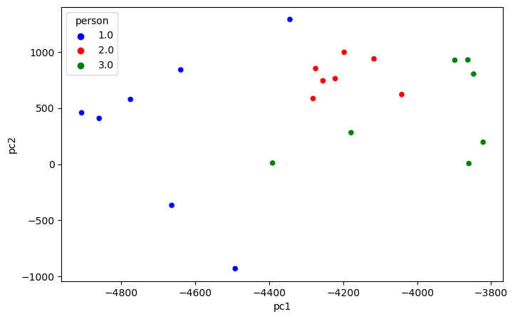

The above plot shows that the data is separable.

Explained variance ratio

s.shape

(280,)

s_norm = s / s.sum()
plt.plot(np.cumsum(s_norm))
plt.xlabel('singular values')
plt.ylabel('cumulative sum')
plt.xlim(0, 280)
plt.ylim(0, 1)
plt.show()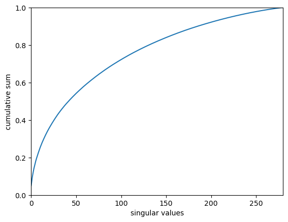

Reconstruct face from top principle components

Original face

picked_face = X_train[0]
show_image(picked_face)

Reconstruct_face method 1

k = 20 # the kth eigenvector

reconstruct_face1 = (picked_face - mean) @ eigen_vecs[:, :k] @ eigen_vecs[:, :k].T + mean
show_image(reconstruct_face1)

Reconstruct_face method 2

S = np.diag(s)
S.shape

(280, 280)

reconstruct_face2 = U[0, :k] @ S[:k, :k] @ (V.T)[:k, :] + mean
reconstruct_face2.shape

(1024,)

show_image(reconstruct_face2)

Confirm the two reconstruct_faces are the same

np.allclose(reconstruct_face1, reconstruct_face2)

True